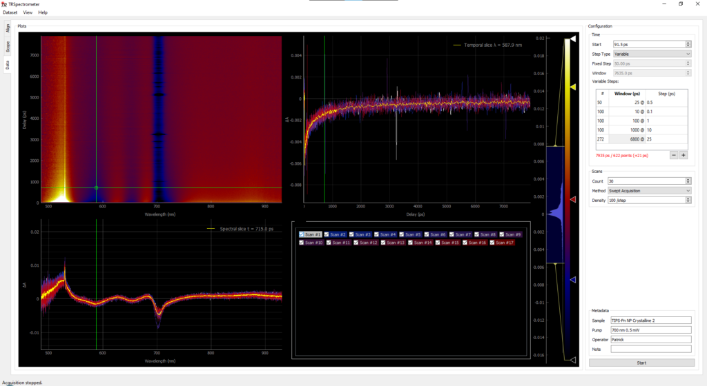
After several months work on both the hardware and software, I’ve finally released version 1.0 of the TRSpectrometer software. This is an open-source platform for time-resolved spectroscopy which I’ve now declared to be in a usable state, fit for public consumption.
The version 1.0 includes a reference hardware design for a transient absorption (pump–probe) spectrometer, along with a full GUI application for the acquisition of data.
Raw data acquisition panel of the TRSpectrometer application.
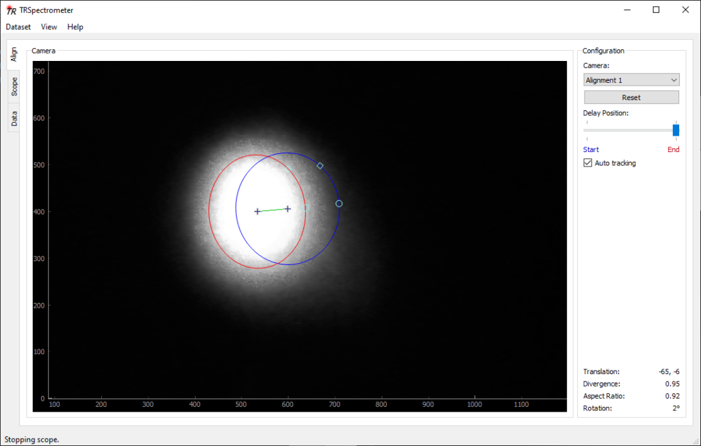
The software features a plugin architecture which allows for flexible additions and modifications to the application. This should make it easy to support different hardware types, experimental methods, or other tools for alignment or data analysis. For example, a plugin is included which uses a webcam and computer vision to assist with alignment of translating delay stages:
Alignment panel plugin for the TRSpectrometer application. A translating delay stage can be aligned with the help of a webcam and computer vision.
The application can be used for data acquisition, or simply for viewing and exploring data. A set of “dummy” hardware devices are configured by default so users can immediately test out some of the acquisition features.
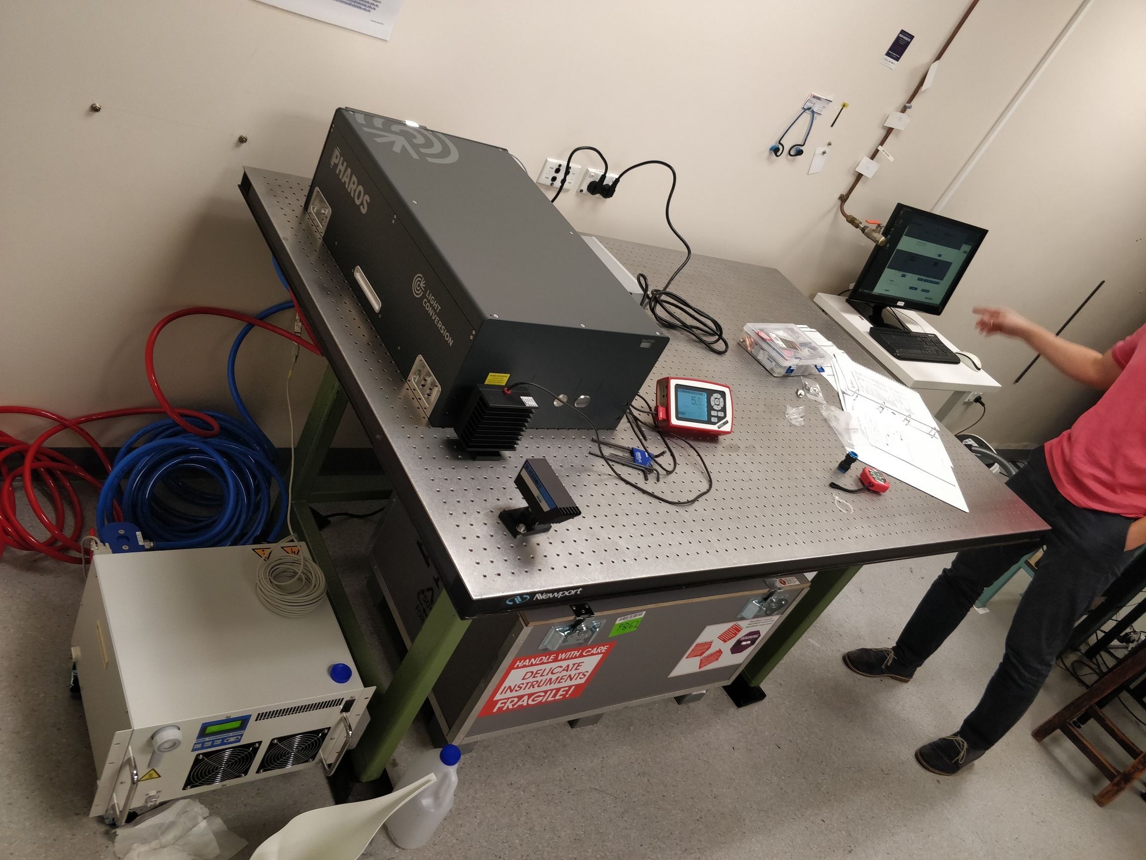
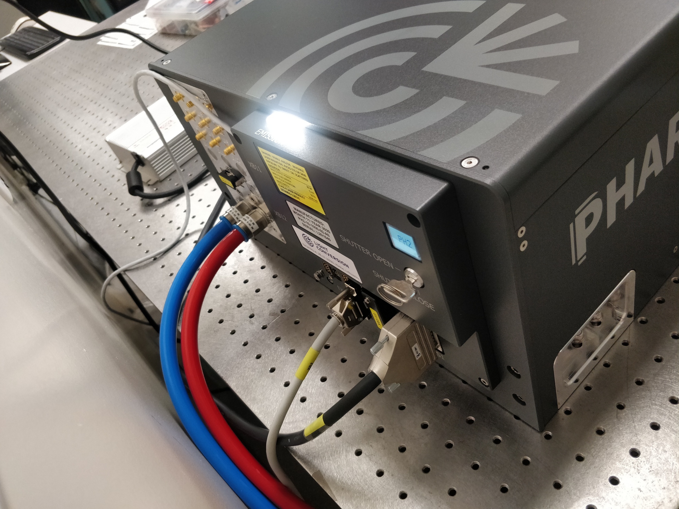
A brand new Pharos laser was installed in the University of Adelaide femto lab today. It’s a pretty nice looking piece of gear manufactured by Light Conversion, and this particular model is so new it’s not even listed on their website at this moment. It emits 10 watts of 1030 nm, with a pulse duration of ~160 fs at a configurable repetition rate of up to 200 kHz.
A Light Conversion Pharos installed in its temporary place in the University of Adelaide femto lab.
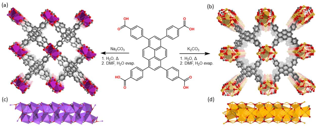
I’m apparently now an expert on metal organic frameworks (MOFs) with the publication of this article in CrystEngComm, DOI: 10.1039/D0CE01505A. In reality, I only worked on the spectroscopy sections — congratulations to Chris who actually touched the chemicals!
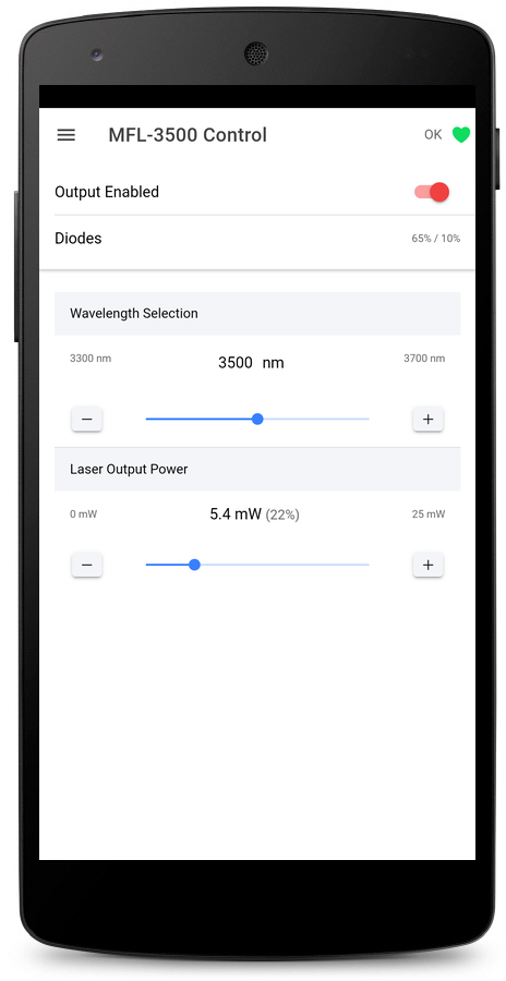
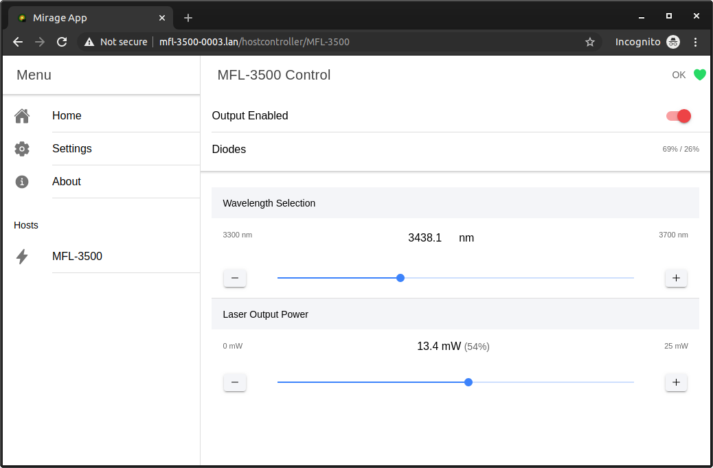
Here’s a quick peek at a project for Mirage Photonics, which is a control interface for their mid-infrared laser system. The laser can be controlled via an Android app or standard web browser interface.
Controlling the MFL-3500 laser via an Android app.Controlling the laser by a web browser interface.
Paper describing the 2D spectrometer design was published in The Journal of Physical Chemistry A (DOI: 10.1021/acs.jpca.0c00285). The accepted version of the manuscript can be downloaded here, along with the supporting information.
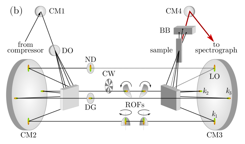
Layout of the 2D spectrometer. CM: concave mirrors, DO: 2-dimensional diffractive optic, ND: neutral density filter, DG: delay glass, CW: chopper wheel, ROFs: rotating optical flats, BB: beam block. The positions of the laser pulses are labeled with kn and LO. The third-order signal (red line) is emitted from the sample on the same path as the LO (dotted line).
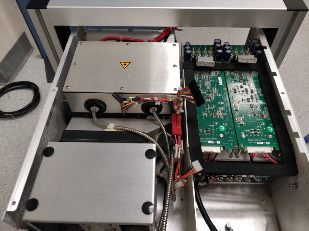
Our Millennia Prime stopped working, tripping the circuit breakers. I’m hoping it’s just power supply issues, and it’s out of warranty, so let’s take a look. Just don’t think about how much this thing costs…
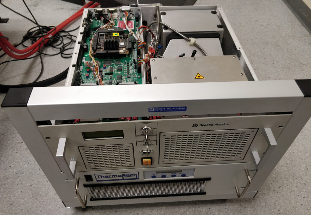
The Spectra-Physics J80 laser diode pump for the Millennia Prime unit, minus top panel.
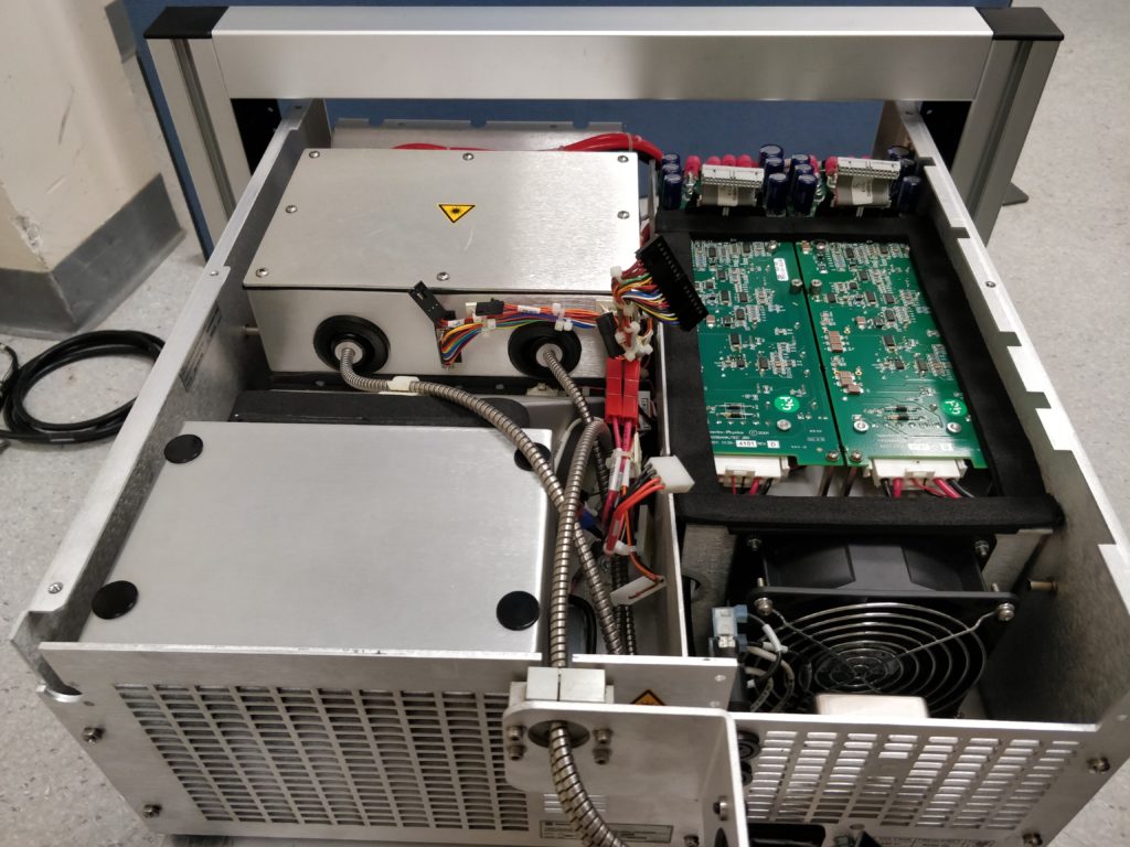
Getting to the power supply unit doesn’t look like fun… It is mounted on the bottom left, underneath a couple of layers of circuitry. At this point it’s impossible to even see what sort of unit it is.
Let’s fast forward through the disassembly and see what it is. This is somewhat awkward and time consuming, but not hard once you know how. (Follow in reverse to see how to do the disassembly.)
That looks a bit scary, but the power supply is out!
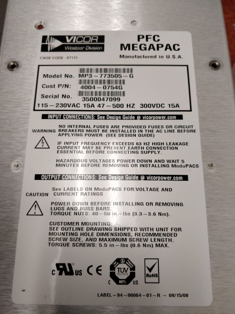
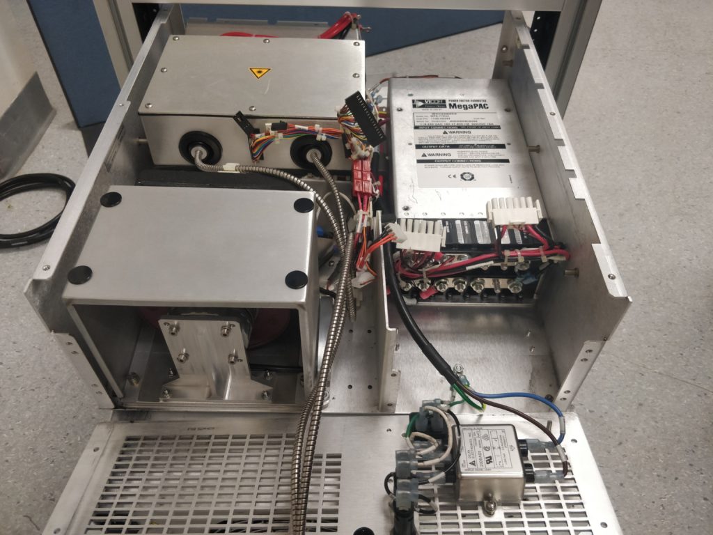
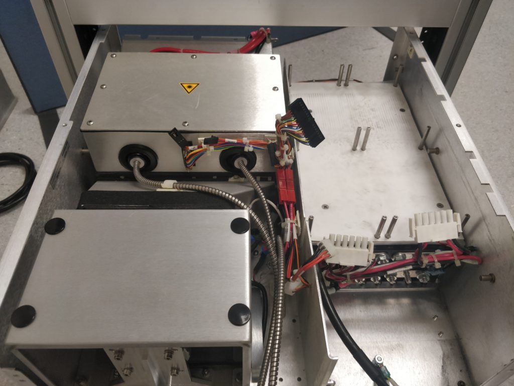
So it’s a commercial unit, a Vicor PFC MegaPAC.
Vicor PFC MegaPAC power supply unit from the Spectra-Physics J80 diode pump laser for the Millennia Prime.
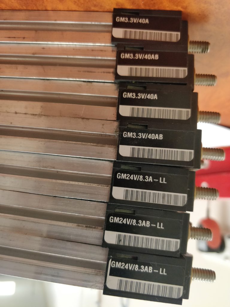
These units are customisable, using a switch mode front-end to produce 300 V DC, which is then converted down to the required voltages using up to 8 DC-DC converter ModuPAC modules. These modules are easily removable.
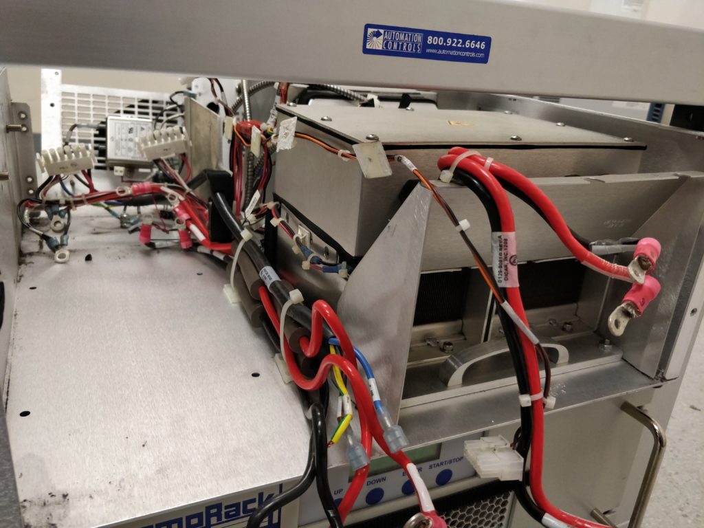
Vicor ModuPAC modules used in the Spectra-Physics J80 diode pump laser for the Millennia Prime.
The unit is set up to use two high-current 3.3 V rails to run the two laser diodes, and a single 24 V rail to run the thermoelectric cooling system and other electronics. The “B” in the model name indicates they are a “current booster” module, and are connected in parallel to the equivalent non-B module. Note that the J40 system only has a single diode, so I would expect it to only have one 3.3 V rail, and perhaps one fewer of the 24 V boosters.
So the Vicor PFC MegaPAC can be bought new, but they are pretty expensive. We’re looking at over $4000 to replace this unit as configured, with at least a 6-week wait time. The DC-DC converter modules are probably fine though, and can be swapped into another front-end… and there’s a few options on eBay. We ended up getting one shipped from the US for just over $300 (yes, about a third of that was shipping costs). The DC converters swapped over fine and a quick check with a multimeter indicates it’s working OK and no longer tripping the circuit breakers.
So here’s the reassembly (the disassembly process is just the reverse of this). Bolt the power supply back into the chassis from the side and bottom.
The Vicor PFC MegaPAC is bolted into the J80 frame from the side and underneath.
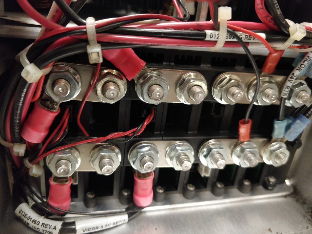
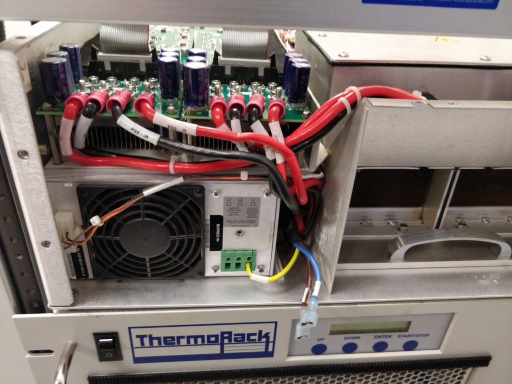
Attach the DC terminals and the voltage trim pot connectors (the small Molex plugs with red and black wires).
DC connections to the Vicor PFC MegaPAC. Two 3.3 V rails and one 24 V rail. The bus bars connect the booster modules to the matching master modules.
Screw in the mounting bracket for the diode driver circuitry onto the top of the power supply.
Mounting bracket is screwed onto the top of the power supply.
Mount the diode driver circuit boards and plug in the connectors at the back. The black foam is to seal this chamber to direct airflow through the power supply and heatsinks on the diode driver boards. Try not to destroy it during disassembly!
The two diode driver modules of the J80. The J40 would just have one of these.
Connect the high-current 3.3 V lines and diodes to the driver boards. Screw in the ground connection to the power supply, and plug in the connector on the left (this is the connection to the logic board to independently switch the 3.3 V rails on or off).
3.3 V and diode connections to the driver boards.
Fit the rear fan assembly using the nuts on the bottom, then re-attach the back panel. The fibre optic cables are armoured, but be careful here and don’t twist or kink them.
Back panel and fan assembly fitted to the J80.
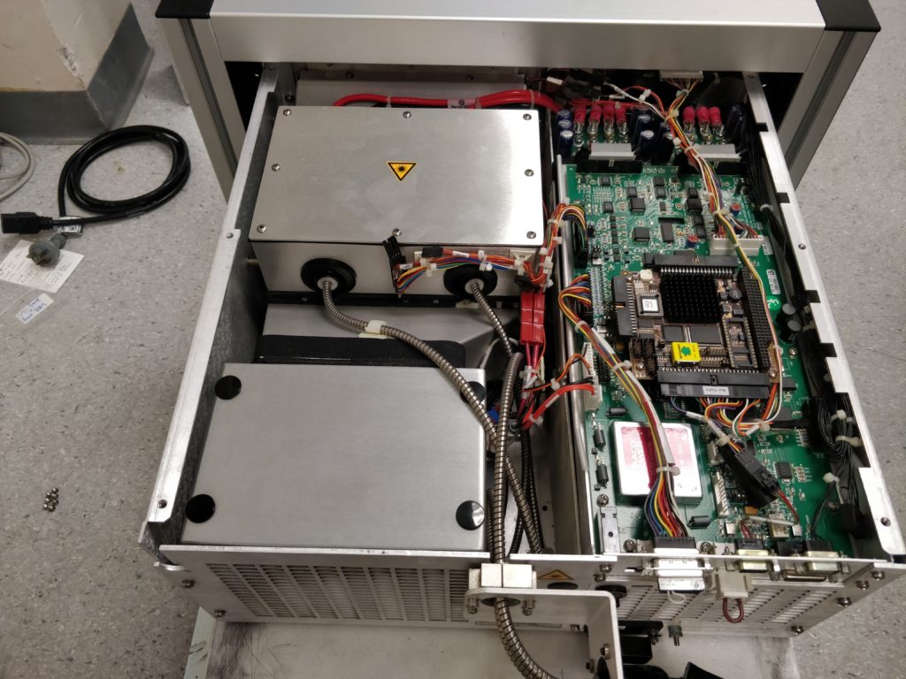
The logic board is then fitted on top of the diode driver boards. Connect the various Molex plugs.
Logic board fitted to the J80.
Note that the rear panel DB-15 connector and the black wires (bottom-right and right side of the above photo, top-right and top of below photo) are actually attached to the front panel. The DB-15 needs to be unscrewed from the rear panel during disassembly.
Logic board fitted to the J80, showing the single-board computer sub-board and 24 V DC-DC power supply module.
As an aside, you can see the single-board computer and 24 V power converter here. That cylinder on the right is a PS/2 keyboard socket. We’ll resist the urge to try hacking it…
Reattach the front panel and connectors to the power switch/power supply, LCD and indicator diodes. The red switch part of the key lock pops out of the lock assembly.
Front panel connections to the J80.
Now put on the top panel, plug it in and fire it up. Yes, it is now working perfectly again!
Update: This post is now outdated! We ended up using a similar, but much improved, spectral interference method using a broadband laser source instead of the continuous-wave HeNe laser. The method is described in the publication on the spectrometer design.
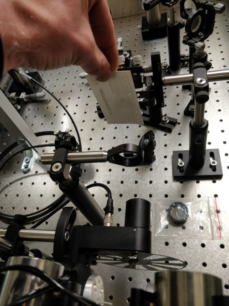
Here is a quick rundown on how the delay stages are calibrated to relate the rotation angle to the delay time of the laser pulse.
An interferometer is built by inserting a mirror/beamsplitter combination after the delays to interfere pairs of the four beams. A Helium-Neon (HeNe) laser is used as the light source, as the atomic emission at 632.8 nm is very well defined — a requirement to make a nice interference pattern and for use in the calibration fit equation.
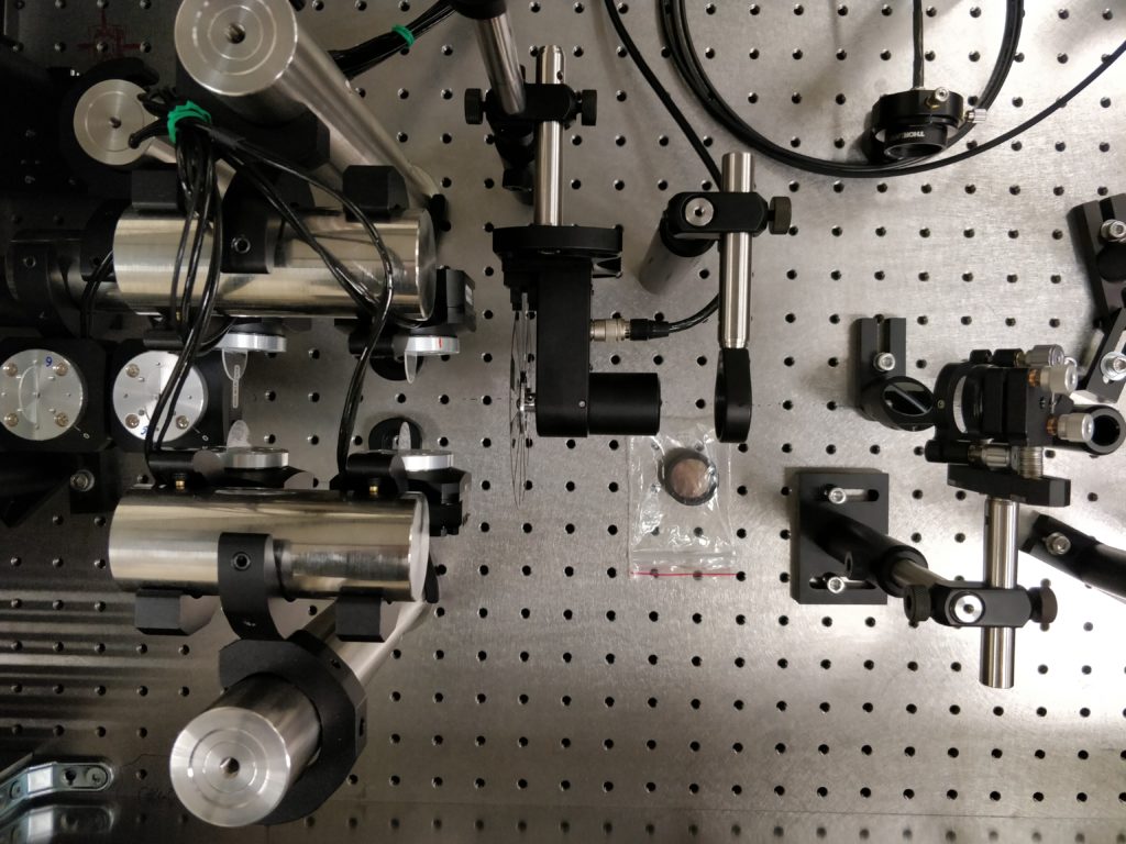
A HeNe laser is used for calibration of the delays.
Three of four HeNe laser spots used for delay calibration.
Here we show the vertical configuration of the beamsplitter/mirror combination, which interferes the top and bottom beams, directing them downwards towards the table. The beam is directed to a fibre-optic which feeds the spectrograph and camera.
Overview of back end of interferometer used for delay calibration, in the vertical configuration.
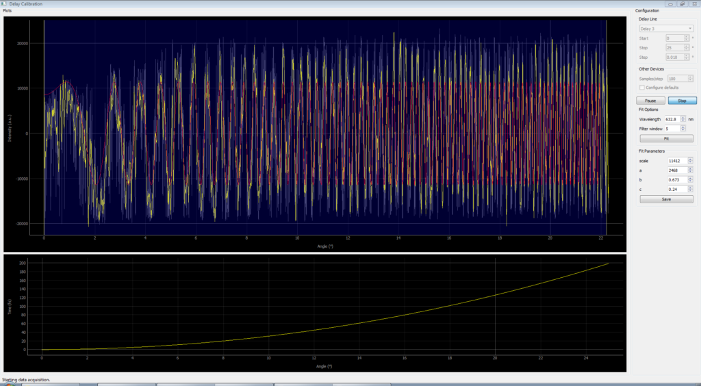
I think this is the first look here at some of the spectrometer software! The intensity at the 632.8 nm laser line is collected as a function of one of the rotational stage angles. The rotational stage is swept between 0° (glass perpendicular to beam) to around 45°. An interference pattern is generated.
Delay calibration interference pattern and fit.
The grey trace is the raw intensity data as a function of rotational stage angle. The yellow trace is with a Savitzky–Golay noise filter applied. The red trace, and the yellow curve in the bottom panel show the theoretical angle-to-delay relationship. As the data is collected, or when the “Fit” button pressed, the fit is performed and the three fitting parameters (α, β, γ) are determined. The fit can also be adjusted in realtime as the parameters are changed manually.
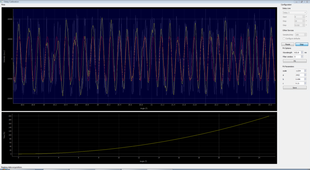
Zoom into part of the collected delay calibration interferogram.
The theoretical model of the glass angle vs delay match the data very well across the entire range of rotation angles. That’s good, as it’s pretty fundamental to the whole spectrometer design!
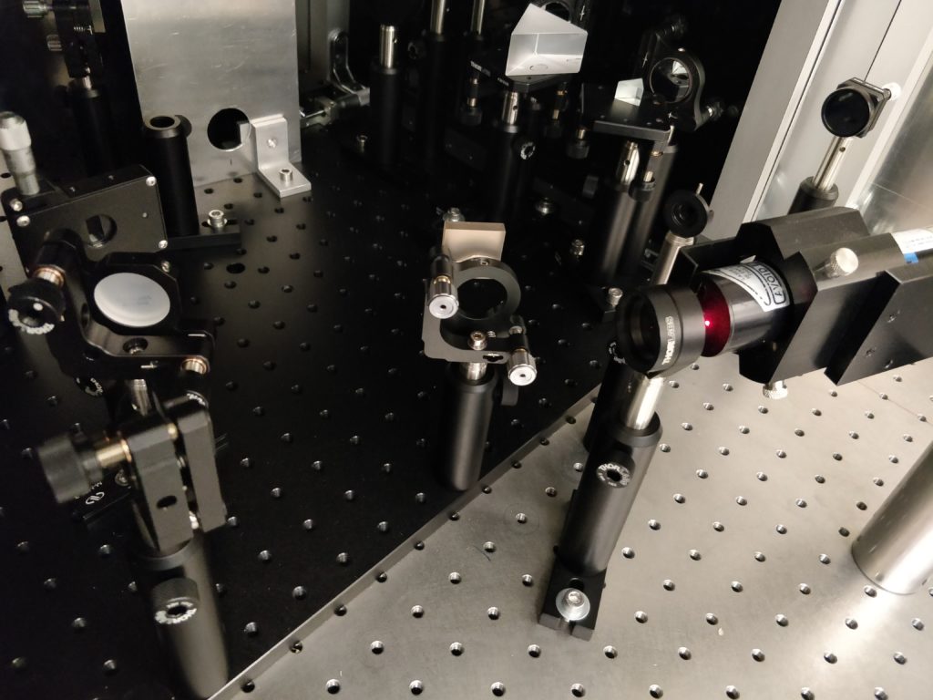
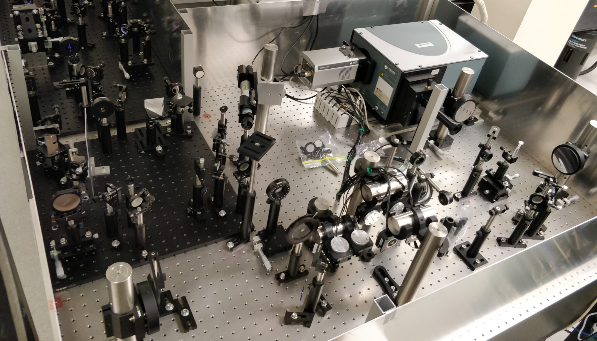
Here’s a nice picture showing an overview of the spectrometer layout. The NOPA is in the back-left, with the compressor on the left. The spectrometer arms run down along the bottom edge, through the delay stages in the bottom centre. The beams are then directed back up to the sample and detector on the right side of the image.
Overview of the NOPA, compressor and 2D spectrometer.
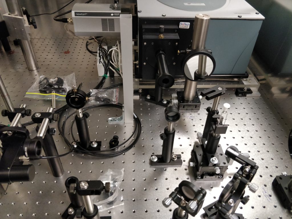
This is the back end of the spectrometer arms. The sample vial is visible, as well as the mirrors and lens used to direct light from the sample into the detector. The spectrograph is an Andor Shamrock, with an Andor Newton CCD camera as the detector. This is able to capture 500 spectra per second.
The output end of the spectrometer, showing the sample and the Andor Shamrock spectrograph and Newton camera used as the detector.